1. Overview
Starting point — the CPU path of GPU code is slow
Run a solver written for the GPU on a CPU and it is slower than code optimised for the CPU from the start, because the data structures and kernel decomposition follow the GPU execution model.
The CPU path cannot simply be dropped, though. It has to run where there is no GPU, it is the reference against which GPU kernel correctness is checked, and debugging during development happens on the CPU.
That is where the question began. How much is recovered by adding OpenMP to the CPU path?
How we ended up at the hybrid
Filling in OpenMP coverage led to the next question. Instead of filling every core with MPI ranks, what happens if we reduce the ranks and fill each one with threads? That is hybrid parallelisation.
The two approaches use the same cores but pay different costs. MPI processes are separate, so every subdomain boundary requires communication and a copy of the data exists per rank. OpenMP shares an address space, so there is neither communication nor duplication, but it pays in barriers between threads, false sharing and lost NUMA locality.
Reducing the ranks looked like it would buy two things.
- Less communication — fewer subdomain boundaries
- Less rank-local preconditioner degradation — coarser ranks mean the preconditioner sees a larger subdomain
For that trade to hold, one premise is needed: OpenMP inside a rank has to come close to MPI. If filling with threads is much slower than filling with ranks, the gain from reduced communication is cancelled out.
One thing nagged. Most CFD codes go pure MPI on the CPU. If the hybrid were that advantageous it would already be in wide use, and since it is not, there must be a reason — we wanted to find out what it was first-hand.
The measurement
The same mesh and the same case were run on 4, 8, 32 and 128 cores in three configurations — pure MPI, pure OpenMP and hybrid — and the wall clock compared.
The subject is the CPU execution path of our in-house CFD solver. The meshes are ONERA M6 (306,577 nodes) and NASA DPW CRM (3,600,000 nodes), and the physics is compressible RANS (Spalart–Allmaras).
2. Implementation scope and environment
Measurement environment
A cluster with 16 cores per socket, 2 sockets (32 cores) per node, and 4 nodes for 128 cores.
The 4-core and 8-core measurements were taken separately on a single-socket, 10-core development machine. The environments differ, so absolute times are not comparable across them; below we compare only the relative difference between pure MPI and hybrid within the same machine.
Implementation scope
Before judging anything we completed the OpenMP coverage first, so that the reason for rejection could not be “the implementation was incomplete.”
| Stage | Effect (8 threads, M6 306k) |
|---|---|
| Parallelised turbulence and point loops + edge renumbering | 55.8 s → 42.7 s (speedup 4.15 → 4.71×) |
| OpenMP in the CPU linear solver | 74.0 s → 41.8 s (−43%, speedup 2.50 → 4.31×) |
The serial fraction back-calculated with Amdahl’s law fell from 38% to about 13%. Pure OpenMP itself, we judged, had done its job.
Partial parallelisation of the linear solver gained almost nothing. Parallelising only the SGS sweep gave a 12% improvement on 8 threads; including SpMV and the vector operations brought it to −33%; and only when the diagonal inverse — which builds 300,000 5×5 inverse matrices at every Newton step — was included as well did it reach −43%.
3. Results
3.1 The winner changes with core count
| Cores | Pure MPI | Best hybrid | Winner |
|---|---|---|---|
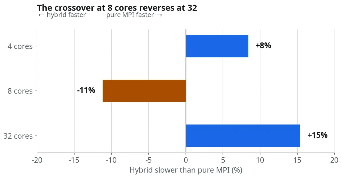
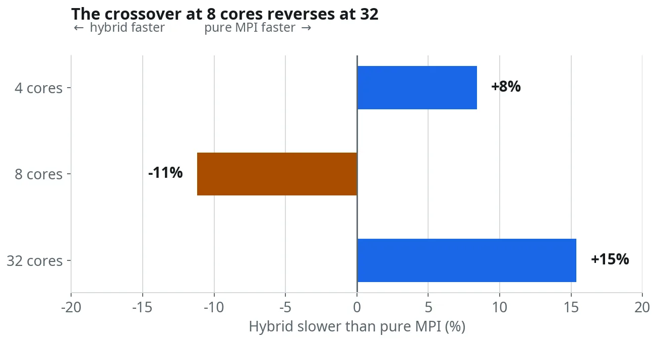
| 4 | 53.24 s | 57.71 s (np2×T2) | MPI +8% |
| 8 | 35.93 s | 31.91 s (np4×T2) | Hybrid +11% |
| 32 | 9.76 s | 11.26 s (np8×T4) | MPI +15% |
Seeing the hybrid lead at 8 cores, we read it as “the hybrid gets more favourable as cores increase.” The 32-core measurement showed that reading to be wrong.
The single-socket, 10-core range was not the range where MPI is strongest but the only range where the hybrid leads at all, and reading it as the start of a trend was the misinterpretation.
3.2 The configuration the design aimed at is the slowest
At all three scales the ordering was np8×T4 > np4×T8 > np2×T16. The figures below are for CRM 3.6M on 32 cores, solver phase only.
| Configuration | Solver phase | vs MPI |
|---|---|---|
| Pure MPI np32 | 312.1 s | — |
| Hybrid np8×T4 | 348.8 s | +12% |
| Hybrid np4×T8 | 396.9 s | +27% |
| Hybrid np2×T16 | 501.2 s | +61% |
The shape the hybrid design was aiming at is one rank per socket (np2×T16). It is the most natural configuration in that it never crosses a NUMA boundary, and it was consistently the slowest of the three.
Smaller thread teams are faster — and the extreme of that is pure MPI.
The hypothesis that there is a wall at the socket boundary was itself correct. Pure OpenMP on 32 cores actually slows down when threads go from 16 to 32 (29.46 s → 30.78 s). But rather than reducing ranks to avoid that wall, increasing ranks so as never to meet it was faster.
3.3 The preconditioner gain does not exist
The second expectation — that fewer ranks make the rank-local preconditioner coarser and improve convergence — was tested on 4 nodes, 128 cores, with SGS used as the preconditioner throughout.
| Configuration | Solver phase | Linear iterations |
|---|---|---|
| Pure MPI 128 ranks | 121.1 s | 1.00 |
| Hybrid 32 ranks×T4 | 127.6 s | 1.00 |
| Hybrid 8 ranks×T16 | 162.3 s | 1.00 |
All three show linear iterations of 1.00: there is no degradation, and reducing ranks improves nothing.
The cause lies in the preconditioner implementation. Block SGS splits the row range per thread and sweeps block-locally, so the number of subdomains the preconditioner sees is ranks × threads — exactly the same as pure MPI. This could have been known by checking the preconditioner implementation before starting.
3.4 Scaling efficiency ranks in the opposite order
Absolute time and strong-scaling efficiency rank in exactly opposite orders.
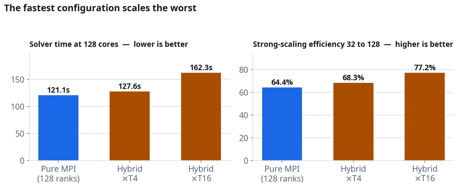
Pure MPI starts from the fastest position and scales worst. Assuming that efficiency holds, the curves cross somewhere around 512 cores.
That extrapolation is an optimistic estimate from two data points, however. Partitioning CRM 3.6M across 2,048 cores leaves 1,800 nodes per rank, so the mesh runs out first. This finding is valid up to 128 cores; beyond that it has to be measured again on meshes of tens of millions of nodes.
4. Why
What the hybrid set out to reduce was communication. At this problem size, communication was not the bottleneck. The parallel efficiency of pure MPI was 44–50% at 32 cores and 64% at 128 — within the normal range.
In exchange for reducing something that was not the bottleneck, we took on barriers inside the thread team, false sharing and lost NUMA locality, and that cost exceeded the gain. The consistent ordering across all three scales — smaller teams are faster — supports this. A thread team costs in proportion to its size, and a team size of one is optimal.
The preconditioner gain never existed. As long as the number of subdomains is ranks × threads, reducing ranks does not make the preconditioner coarser.
5. What to check in the measurement
These are the traps we actually fell into. Get the measurement wrong and the conclusion inverts.
| Trap | Symptom |
|---|---|
The solver reporting time with clock() | clock() is the sum of CPU time over all threads, so the value grows with thread count. It produced the false observation that “parallelising makes it slower” when the actual speedup was 4.88× |
| OpenMP threads not pinned | The scheduler piles threads onto hyperthreading sibling cores and the effective core count halves |
| Missing binding in MPI hybrid runs | With --bind-to none, every rank occupies the same physical cores. The difference is 93.07 s against 31.91 s — 2.9× — and measuring in that state yields the opposite conclusion, “the hybrid is useless” |
Measuring memory with maxRSS | It is the peak of a single process, so it does not give the MPI node total |
ps -C / ps comm | Process names are truncated at 15 characters. Two builds became indistinguishable and every measurement came back zero |
| Judging on total wall clock | Differences in setup time get mixed in. In a real 30,000-iteration run, setup is 0.4% of the total |
The first item matters most. Every measurement taken before it was fixed was invalid.
6. Conclusions
Pure MPI appears to be the better choice on performance alone, before the development and maintenance cost of the hybrid is even counted.
That is the conclusion after completing the OpenMP coverage, parallelising the linear solver as well, and measuring at four scales. Of the two gains the hybrid was expected to deliver, the speed gain was a local phenomenon at 8 cores, and the preconditioner gain never existed given how the subdomain count is formed.
The answer to the question we started from — how much of the CPU path of GPU-oriented code can be recovered with OpenMP — is “it is effective as far as cutting the serial fraction to 13%, but filling those cores with MPI ranks is still faster.”
And there is a reason most CFD codes go pure MPI on the CPU: a thread team costs in proportion to its size, and a team size of one is optimal.
Others reached the same conclusion first. The linear algebra library PETSc also attempted to add an MPI+threads hybrid, but performance was often worse than the MPI-everywhere approach despite the added code complexity, so hybrid support was removed and PETSc uses MPI only (Frustrated with MPI+Threads?, 2024). The 2016 PETSc meeting even included a talk titled To thread or not to thread? Why PETSc favors MPI-only.
There are reports in the other direction, though. Results published for PETSc show that as node counts grow, the subdomain per rank coarsens and the hybrid becomes favourable (arXiv:1303.5275). That points the same way as the scaling-efficiency inversion observed in §3.4, and it shows that the question is not which side is right but at what scale you measure. It is also why this article limits its finding to 128 cores.