1. Overview
Background
One of the recurring chores of a CFD engineer is finding an appropriate CFL number. CFL governs the trade-off between convergence stability and computational cost, and its optimum varies widely with the mesh and the flow condition. It is worse in compressible analysis, where the initial transient, shocks and separation make the residual behaviour change abruptly. Set it low and the run is slow; set it high and it diverges.
The result is a reliance on the engineer’s experience and intuition, which is a wall for both reproducibility and automation.
Limits of existing automation
Automated CFL techniques already exist.
- CFL Adaptive (heuristic) — adjusts CFL automatically from residual indicators. It has many parameters to tune, and a safe setting makes aggressive convergence hard to obtain.
- CFL Ramp (scheduling) — follows a fixed schedule set in advance. Get the values wrong and it diverges easily.
Both react to the instantaneous residual or follow a preset, and never see the convergence trajectory as a whole. A human, by contrast, looks at the residual history and judges “this is a plateau, we can push it up.” Whether an LLM can make that judgement instead is the starting point of this study.
Objective
To verify whether CFL can be controlled dynamically on a single grid, without multigrid and without fine-tuning, using nothing but a commercial LLM.
2. Control system
2.1 Observe, decide, actuate interface
Solver internal state (iteration, residuals, CFL) is streamed to an external client, and an external controller injects the CFL for the next interval through set_cfl. The solver algorithm is untouched; only a thin runtime control layer is added from outside.
One more mechanism was added: pause-during-inference, which halts the solver while the LLM is reasoning. This applies the decision to exactly the state that was observed, and in particular prevents the state from deteriorating further while a response is awaited once divergence has begun.
2.2 The LLM agent control loop
On a time-based interval (about one minute by default), a window of residual history over the last N iterations is passed to the LLM, and the CFL value returned as structured output is injected into the solver’s outer loop.
- Receive the residual history window (last N iterations)
- LLM decision —
{cfl, rationale} - Safety post-processing — clamp to upper and lower bounds, limit the rate of change against the previous value
- Apply
set_cfland hold until the next interval
Decisions are made on the trend of the residuals — decreasing, plateauing, oscillating — rather than the instantaneous value (explore-then-hold). A multi-turn memory was also added, feeding the agent’s own decision history back into the stateless API so that it remembers CFL values that previously diverged and avoids retrying them.
2.3 The two-timescale hybrid
The LLM has a latency of seconds and a per-call cost, so it cannot be a safety controller that acts every iteration. The layers were therefore split by timescale.
| Layer | Interval | Role |
|---|---|---|
| Fast safety layer (rules) | about 1 s | On detecting divergence, immediately CFL × 0.6 |
| Slow strategy layer (LLM) | about 1 min | Search for and hold the moving optimum CFL |
There is a physical basis for this. The ceiling of the stable CFL is a time-varying quantity that rises as the flow settles. A static memory that permanently forbids a CFL that once diverged is therefore harmful, and the multi-turn context was designed to handle that time dependence.
3. Analysis setup
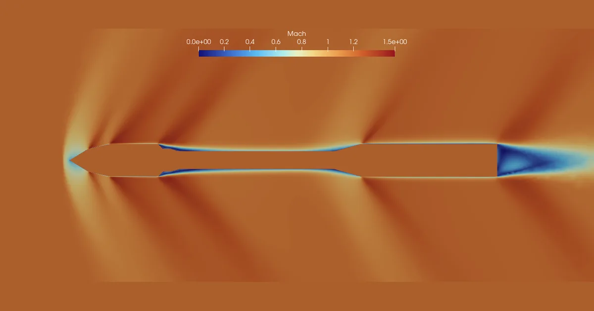
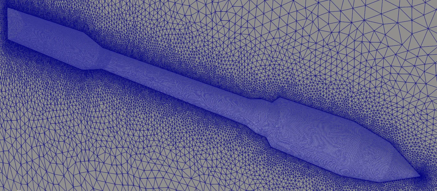
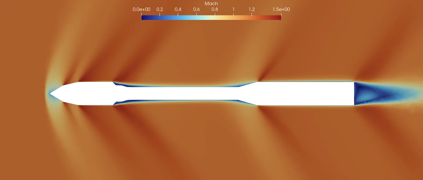
- Target: Taurus launch vehicle, hammerhead configuration
- Conditions: M∞ = 1.187, α = 2.0°
- Analysis: steady compressible RANS (SA)
- Solver: Wake, our in-house GPU-native CFD code
Three LLM configurations were compared.
- A — multi-turn memory
- B — memory + reasoning (thinking)
- C — memory + reasoning + safety layer (the two-timescale hybrid)
The baselines are Constant, Scheduled Ramp (mild/aggressive) and Adaptive (heuristic).
4. Results
4.1 Conventional CFL methods
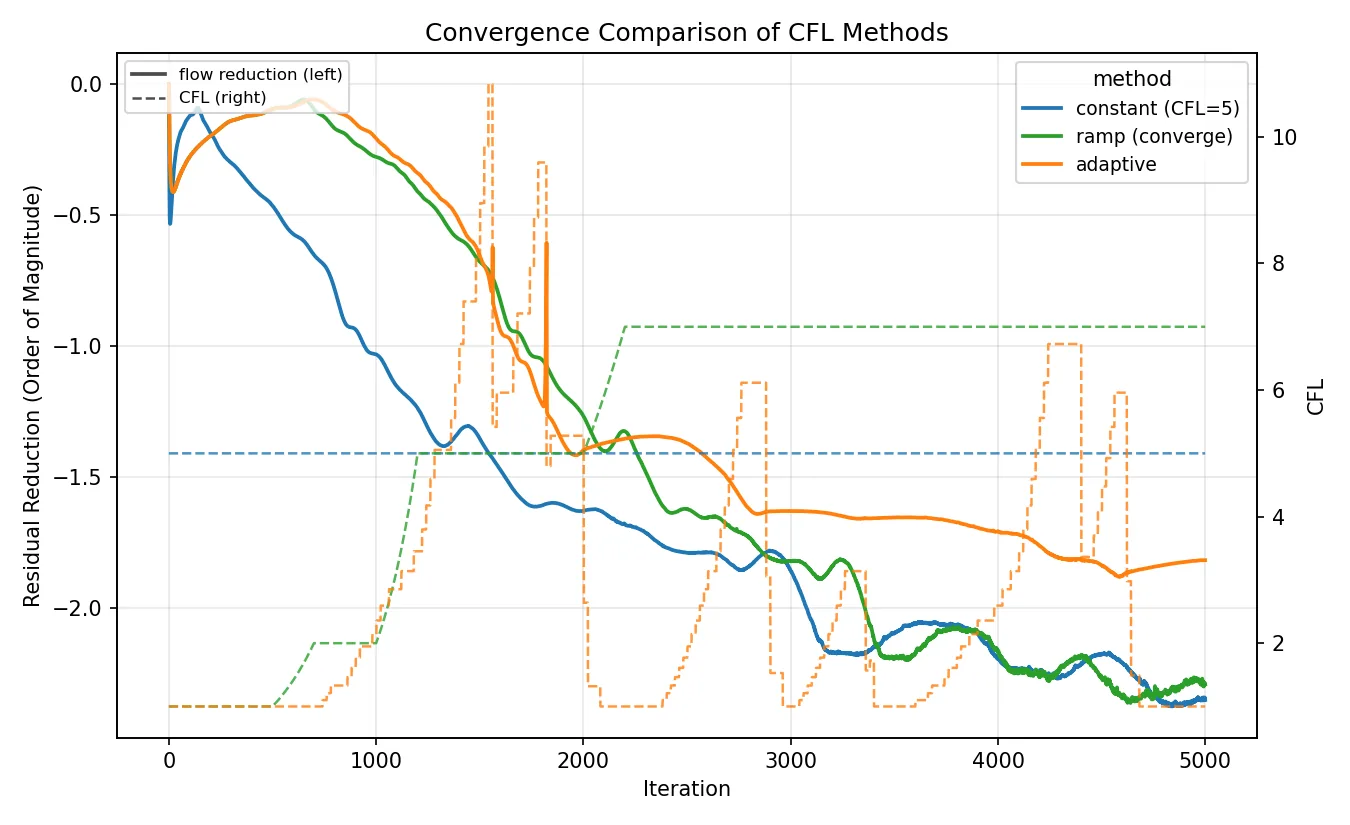
Constant CFL 5 was slow but converged deepest, reaching a log reduction of −2.18. Ramp (mild), raising CFL from 1 to 7, converged similarly (−2.09); Adaptive (heuristic) behaved conservatively and stalled at −1.62 as its CFL fell late in the run.
The human-set constant CFL is the baseline — the line the LLM has to beat.
It is worth adding that CFL affects only convergence speed and stability: the converged final solution was independent of the CFL control method.
4.2 The LLM alone
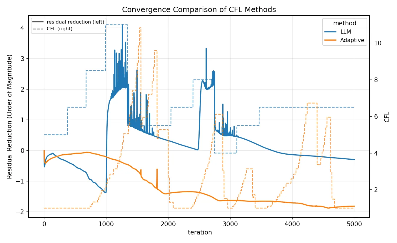
The LLM raised CFL aggressively at the start to search for the optimum, and over that stretch it led the baseline. But it repeatedly exceeded the time-varying stability ceiling, and overshoot followed by collapse recurred like an oscillation. The final log reduction was −0.125, short even of the heuristic Adaptive.
There are three causes.
- Control latency — the API interval, plus the time taken to recognise a collapse
- Overreaction — cutting CFL too far once the collapse is recognised
- Ceiling re-search — pushing back up after the cut and repeating the same process
4.3 LLM + reasoning
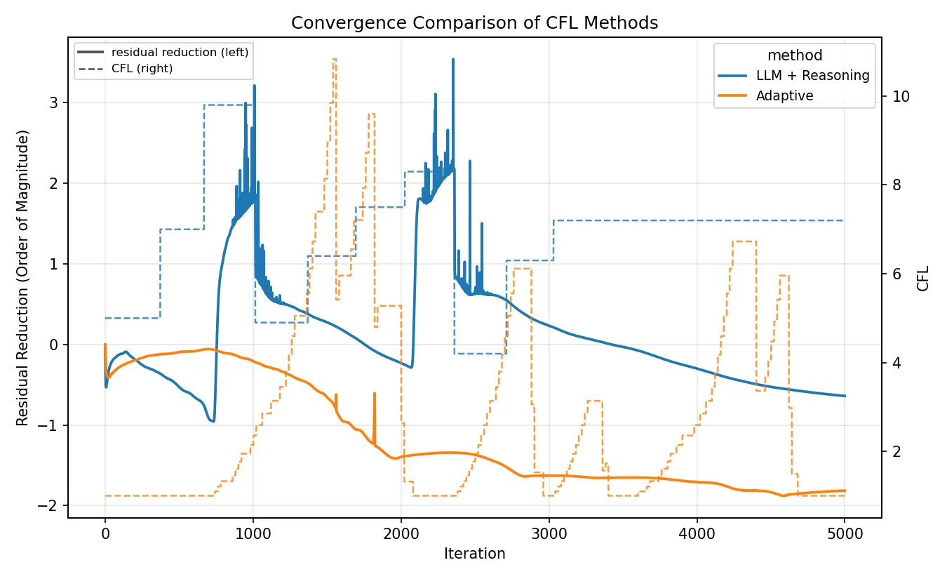
Adding reasoning (thinking) improved decision quality and eased the oscillation somewhat. The fundamental problem of slow, after-the-fact recognition, however, was not solved. The final log reduction was −0.471, still below the heuristic Adaptive.
Making the model think harder is not enough on its own; a separate safeguard that responds quickly to divergence is required.
4.4 The hybrid
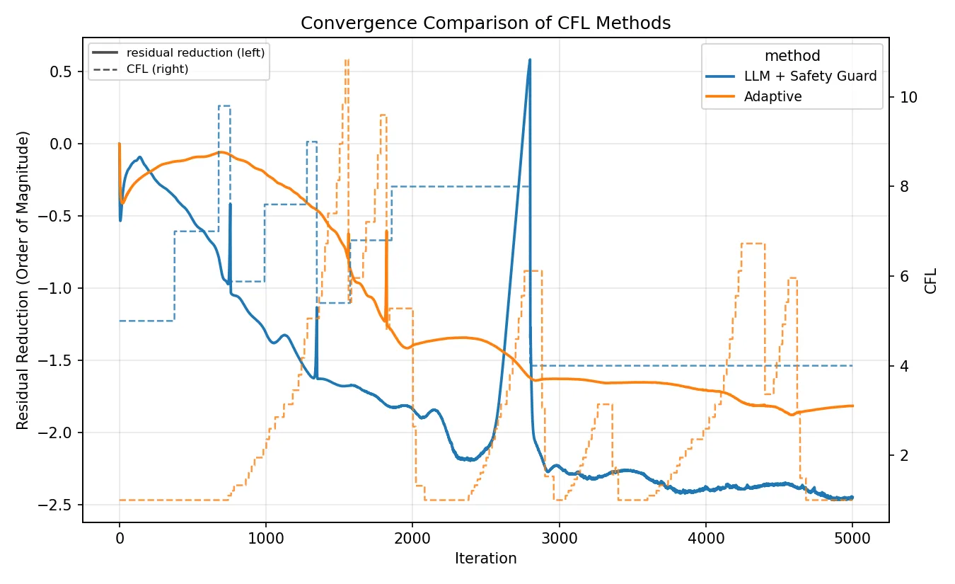
Attaching the rule-based safety layer reversed the result. When an overshoot occurred, the rule cut CFL from 9.8 to 5.88 within 79 iterations, so the controller tracked the optimum without collapsing.
The final log reduction was −2.28, beating Constant (−2.18), and reaching a residual of −2 took 2,208 iterations against Constant’s 3,042 — about 27% fewer.
4.5 Summary
| Method | Final CFL | log₁₀Res | Reduction | iter → 1e-7 | Status |
|---|---|---|---|---|---|
| LLM + safety guard | 4.00 | −7.521 | −2.280 | 2,208 | converged |
| Constant | 5.00 | −7.421 | −2.180 | 3,042 | converged |
| Ramp (mild) | 7.00 | −7.334 | −2.093 | 3,342 | converged |
| Adaptive (heuristic) | 1.00 | −6.861 | −1.620 | — | partial |
| LLM + reasoning | 7.20 | −5.712 | −0.471 | — | partial |
| LLM | 6.50 | −5.366 | −0.125 | — | partial |
| Ramp (aggressive) | 8.00 | −2.672 | +2.569 | — | diverged |
5. Conclusions
We confirmed that CFL can be controlled dynamically on a single grid with a commercial LLM and no fine-tuning. The automation works. A controller can take over the process by which an engineer hand-searches for a CFL, and the hybrid configuration converged both deeper and faster than a human-set constant CFL.
The result needs to be read precisely, though. What produced the stability was the rule-based safety layer, not the LLM. Both the LLM alone and the LLM with reasoning fell short even of the heuristic Adaptive, and only once a rule running every second was attached did the configuration beat the baseline. What the LLM contributed was the strategic judgement of finding and holding the moving optimum CFL, and that sits on top of the rules rather than replacing them.
Cost has to be counted too. This configuration calls an API roughly once a minute and halts the solver during inference because of the latency. A delay of seconds is unusable in the first place for safety control that has to make a decision every iteration. If what you gain is a 27% reduction in iterations, that has to be weighed against the call cost, the latency, and the added external dependency.
In summary:
- As a means of automation it works. It replaces the human’s repeated search and can beat a well-tuned manual setting.
- As a replacement for the algorithm it is expensive. For control that must act at every step, rules are far cheaper and faster, and an LLM cannot stand in for that layer.
Rather than pushing an LLM inside the CFD solver, separating the layers — strategic judgement outside the solver, rules inside — looks like the realistic design for now.