CFD of an S-Duct Intake — Steady State Flow

1. Overview

This study evaluates the aerodynamic performance of a stealth aircraft S-duct using Flow360, a next-generation GPU-native CFD solver. Massively parallel GPU computation resolves the complex three-dimensional steady flow inside the duct quickly and accurately, making efficient performance prediction possible at an early design stage.

Background

The S-duct is a key component for reducing the radar cross-section (RCS) of a stealth aircraft, but the complex curved geometry that lowers RCS carries a conflicting penalty in aerodynamic performance. Secondary flow and vortices produced by the duct curvature deepen the total pressure loss and flow distortion of the air entering the engine. That is a direct cause of thrust loss and operational instability.

The procedure for generating S-duct geometry and the method for quantifying AIP flow distortion are covered in a separate article. This article focuses on which solver to use for the same flow.

The problem

Predicting the complex flow inside an S-duct accurately calls for high-fidelity analysis. Conventional CPU-based analysis, however, is very expensive and can take several hours for a single geometry, which imposes real limits in practice. Reviewing a range of geometric variables during aircraft development, or searching for an optimal design, has therefore been difficult.

The approach

Recent advances in GPGPU technology have drawn attention as a way around the high computational cost of conventional CFD. We therefore analysed the flow inside the S-duct with Flow360, a GPU-native CFD solver, alongside CFX, which is widely used for turbomachinery. Flow360 is optimised for the GPU and can reproduce complex flow phenomena quickly and efficiently; the aim of this study is to verify the accuracy of the solver.

2. Domain and mesh

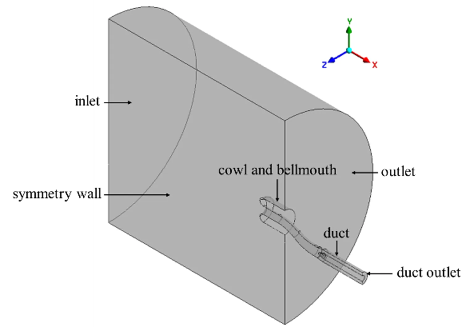
The model is based on the S-duct geometry designed and tested at ONERA (Fig. 1), and consists of a bellmouth that stabilises the incoming flow, an inlet duct, the S-duct itself and an exit duct. To save GPU memory and improve efficiency, flow symmetry was assumed and only half of the domain was solved.

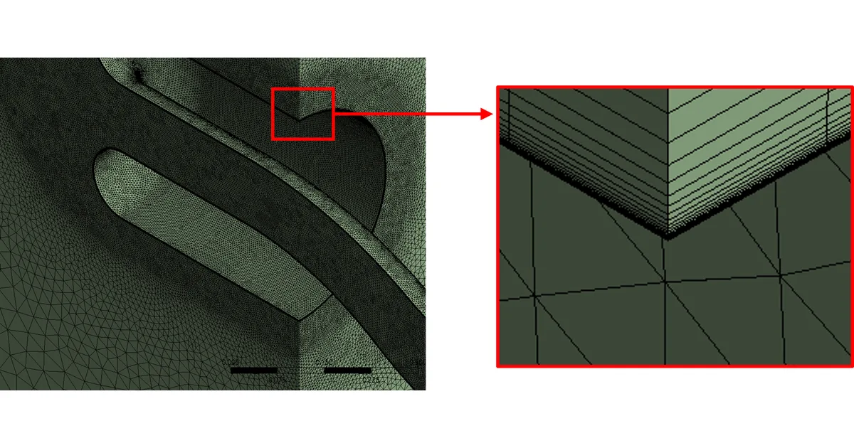
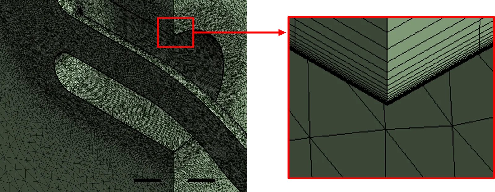
Fig. 1 Computational domain for the ONERA S-duct

The mesh is refined at the bends inside the S-duct and near the walls so that the vortex structures and pressure fluctuations arising from separation and in the wake are captured accurately (Fig. 2). After a grid dependence study, the final mesh had about 3.14 million nodes and 11.63 million elements. For details of the geometry and the experimental setup, see the papers by Delot et al. (2) and Ahrabi et al. (3).

Fig. 2 Computational mesh around the S-duct

3. Results

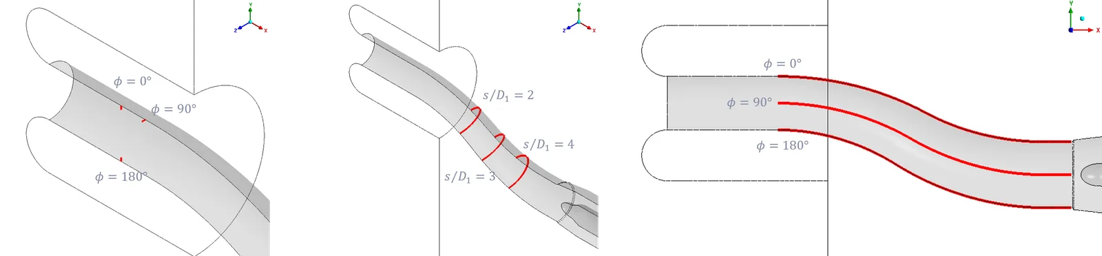
To assess the validity of the numerical approach, the results were compared against experimental data. The comparison uses the pressure distributions measured at the three locations shown in Fig. 3.

Fig. 3 Pressure tap locations in the S-duct

The velocity distribution on the symmetry plane develops as shown below.

Inlet boundary layer profile

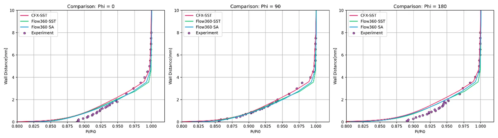
To check how accurately the inlet flow is reproduced, the boundary layer profile was compared against the experiment. As Fig. 4 shows, both the SST and SA turbulence models follow the measured trend, and the performance is on par with other CFD solvers. This confirms that the mesh and numerical scheme used here reproduce the S-duct inlet boundary layer adequately.

Fig. 4 Boundary layer profiles at s/D1 = 0.575

Total pressure across duct cross-sections

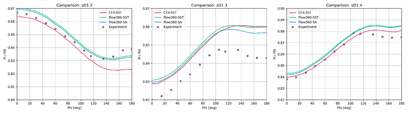
To validate the internal flow, circumferential pressure distributions at three stations inside the duct were compared against measurement (Fig. 5). The computed results follow the experimental trend at every station, and in particular reproduce the pattern in which secondary flow leaves the lower part (Φ = 0°) at low pressure and the upper part (Φ = 180°) at high pressure. Flow360 therefore reproduces the principal flow features of the S-duct reliably.

Fig. 5 Circumferential pressure distribution at three cross-sections

Streamwise pressure distribution

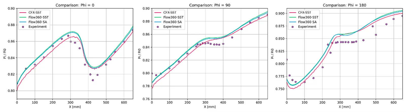
Fig. 6 compares the streamwise wall static pressure against measurement at three locations (Φ = 0°, 90°, 180°). The computed results follow the experiment at every location, reproducing in particular the sharp pressure drop and recovery at the first bend (X = 200–400 mm) and the pressure variation after the second bend. Flow360 thus predicts the flow acceleration and deceleration that follow the change in curvature, and the associated pressure variation, reliably.

4. Conclusions

This case study confirms that Flow360 can accurately predict the complex steady flow inside an S-duct. The predicted pressure distributions agree well with measurement at the key locations, showing that a GPU-native CFD solver reproduces the essential flow characteristics of an S-duct effectively and within a short turnaround.

References

FlexCompute, Inc. (2022). Flow360 Aerospace Applications. Retrieved August 15, 2025, from https://www.flexcompute.com/flow360/aerospace/
Delot, A. L.; Scharnhorst, R. (2013). “A Comparison of Several CFD Codes with Experimental Data in a Diffusing S-Duct,” 49th AIAA/ASME/SAE/ASEE Joint Propulsion Conference, AIAA 2013-3796.
Ahrabi, R. B.; Sreenivas, K.; Webster, R. S. (2013). “Computational Investigation of Compressible Flow in a Diffusing S-Duct,” 49th AIAA/ASME/SAE/ASEE Joint Propulsion Conference, AIAA 2013-3601.