1. Overview
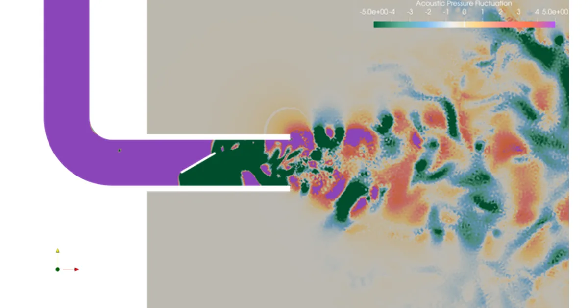
This case study uses Flow360, a next-generation GPU-native CFD solver, to analyse aerodynamic noise in an HVAC system. Flow360 resolves unsteady flow quickly and accurately through massively parallel GPU computation, which makes it cost-effective to study the main sources of HVAC aeroacoustic noise.
Background
As vehicle electrification accelerates, engine noise and the structural vibration that comes with it have fallen sharply. Secondary noise sources that used to be masked by the engine are now significant factors in passenger comfort. Aerodynamic noise generated inside the automotive HVAC system is a prime example.
Beyond the blower itself, flow separation and vortices caused by structures inside the duct produce broadband noise, and in some cases tonal noise as well. This has a direct effect on the acoustic quality of the cabin.
The problem
HVAC noise analysis has traditionally relied on anechoic chamber testing or on coupling high-fidelity CFD with an acoustic solver. Conventional CFD–acoustic coupling, however, is very expensive to compute, and there are real limits to exploring design concepts with it at an early stage. Reviewing several duct geometries or optimising across operating conditions has therefore been difficult.
The approach
Recent progress in GPU computing has made massively parallel computation practical, and both the cost and the turnaround of CFD analysis have fallen substantially. We therefore set out to predict aerodynamic noise inside an HVAC system directly with Flow360, one of the GPU-native CFD codes. Flow360 is optimised for unsteady flow analysis and can capture the complex flow inside the duct along with the noise generation mechanisms that follow from it.
2. Geometry and grid
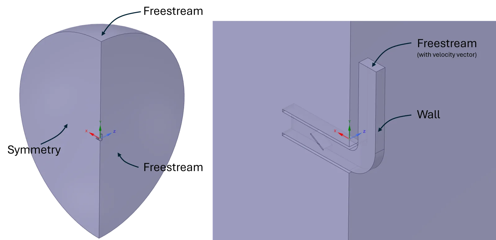
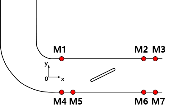
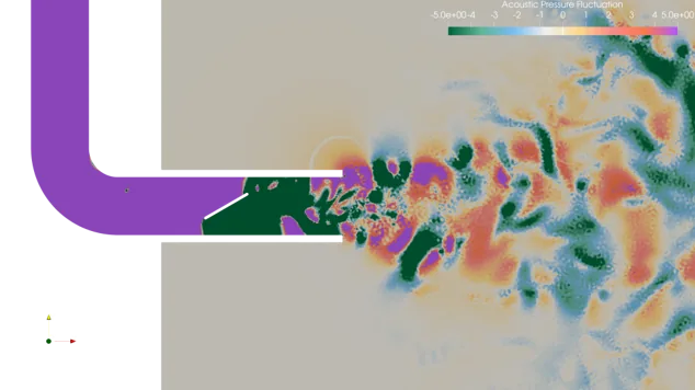
The model used here comes from a study led by a consortium of German automotive companies. It is a rectangular duct with a 90-degree bend and a flap installed inside to generate vortices. To reduce GPU memory the computational domain was simplified to a half-sphere (Fig. 1), and microphones were placed on the duct wall around the flap so that noise can be measured (Fig. 2).
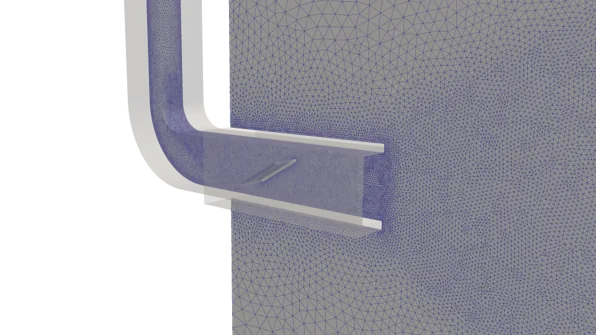
The mesh is particularly dense at the inner bend, around the flap and in the exit region, so that the vortex formation induced by the flap and the resulting pressure propagation are captured accurately (Fig. 3). For details of the experimental configuration and the numerical method, see the paper by Jäger et al. (1).
3. Solver settings
The flow and pressure fields were computed with an implicit LES turbulence model. Flow360 is a density-based, GPU-native Navier–Stokes solver; the specific schemes used here are as follows.
Grid and discretisation
- Grid system: node-centered unstructured grid
- Numerical method: second-order finite volume method
- Convective terms: Roe Riemann solver
- Viscous terms: central difference method
- Spatial discretisation: MUSCL extrapolation
Time discretisation and run conditions
- Time step: Δt = 1.0 × 10⁻⁴ s
- Hardware: two NVIDIA A10 GPUs
- Runtime: about 6 hours for 9,600 steps (0.96 s of physical time)
4. Results
The sound pressure spectra agree well with the experiment across the whole frequency range, which suggests that Flow360 reproduces the vortices generated by the bend and the flap properly.
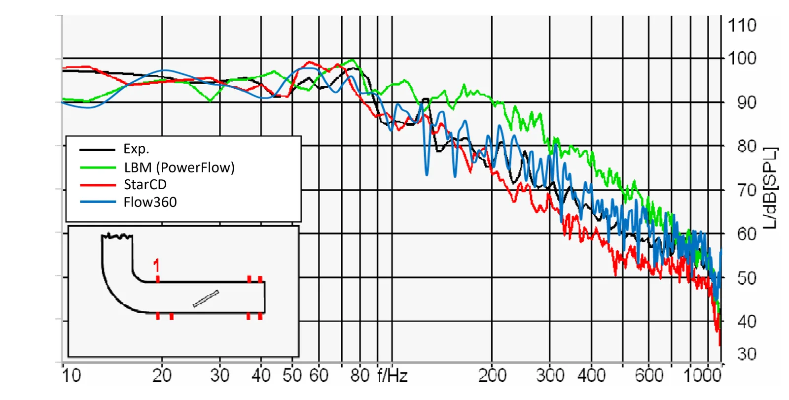
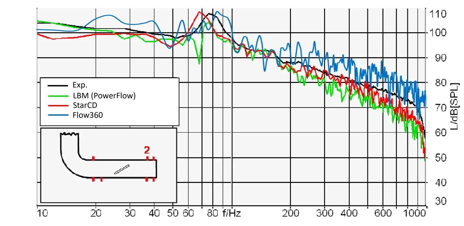
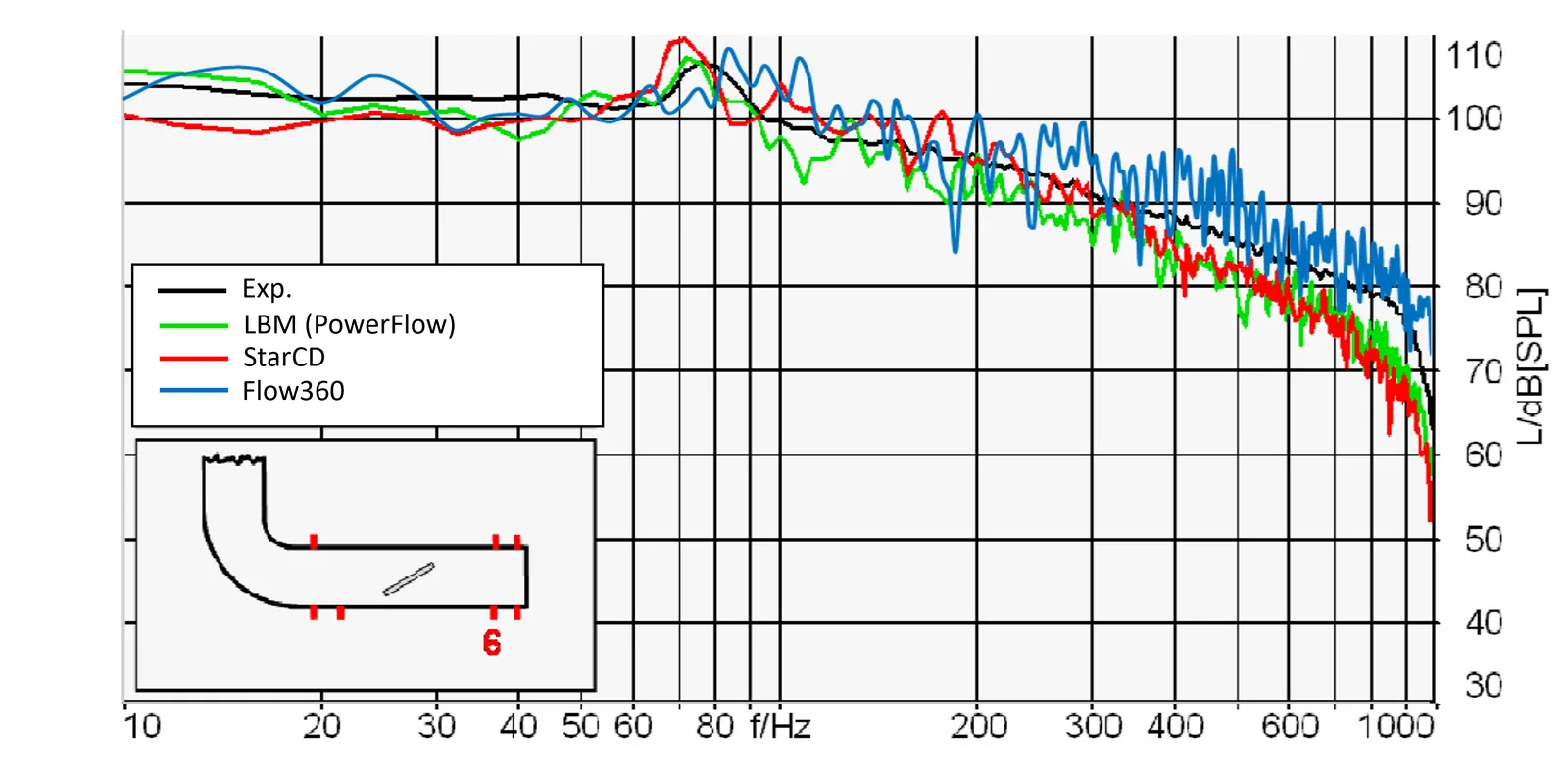
Some discrepancy appears below 100 Hz — at microphone 2 the difference reaches about 5 dB at the 25 Hz bin. This is most likely because the short sampling time makes high accuracy hard to achieve at very low frequencies. Even so, the peak near 80 Hz is predicted correctly at every microphone.
Above 100 Hz in particular, the broadband noise characteristics track the experimental curve very closely, and the prediction is notably better than that of other CFD codes.
5. Conclusions
This case study indicates that Flow360 can predict noise generated inside an HVAC system with reasonable accuracy. The sound pressure spectra predicted at the measurement points closely resemble the experimental values, which demonstrates that a GPU-native CFD solver can simulate aerodynamic noise effectively within a short turnaround.
References
- Anke Jaeger, Friedhelm Decker, Michael Hartmann, Moni Islam, Timo Lemke, Joerg Ocker, Volker Schwarz, Frank Ullrich, Bernd Crouse, Gana Balasubramanian, Fred Mendonca and Roger Drobietz. “Numerical and Experimental Investigations of the Noise Generated by a Flap in a Simplified HVAC Duct,” AIAA 2008-2902. 14th AIAA/CEAS Aeroacoustics Conference (29th AIAA Aeroacoustics Conference). May 2008.
Want to know more about Flow360? Flow360 product page · Flexcompute documentation